Another common mistake in least squares fitting

On p. 121 of Eloquent Science, I spend a page discussing the misuses of linear correlation. Turns out I didn’t cover all of them.

Mark Hibberd writes:

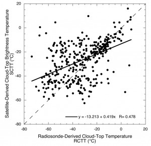
I think your Figure 11.10 [to the right] clearly shows a very common mistake of inappropriately using a standard least squares fit. The fit given (y = -13.2 + 0.42 x) assumes that there is no uncertainty in the y values. Eye-balling the data, it is clear that the line is not a good fit.

If you swap the axes and redo the standard least squares fit you get a fit that would be shown the figure as y = 36.0 + 1.89 x, which is even worse. (I digitised the figure to do the fitting.)

The correct method is to use a bivariate fit, which allows for uncertainty in both x and y. If we assume equal uncertainty in both x and y values, we get y = -2.1 + 0.75 x.

This method is well explained by Cantrell, C.A. (2008) “Technical Note: Review of methods for linear least-squares fitting of data and application to atmospheric chemistry problems” Atmos. Chem. Phys., 8, 5477–5487. He also includes a very useful spreadsheet in supplemental material available with the paper, which I strongly recommend to all scientists who fit data.

Note that a useful warning sign of problems is if fitting x vs y and y vs x give different standard least square fits.

Thanks, Mark, for the advice. For what it’s worth, in the figure in question, we weren’t expecting a great fit to the data, no matter the method. Nevertheless, our inclusion of the regression line should have been done appropriately, regardless.